Overview

The project CHRIS/Proba Toolbox for BEAM (CHRIS-Box) has been brought into life in order to support users of data of the CHRIS sensor onboard of the ESA Proba platform. BEAM and the CHRIS-Box are user tools which ESA/ESRIN are providing free of charge to the Earth Observation Community. The CHRIS-Box software provides extensions for BEAM, which allow accomplishing the following tasks:

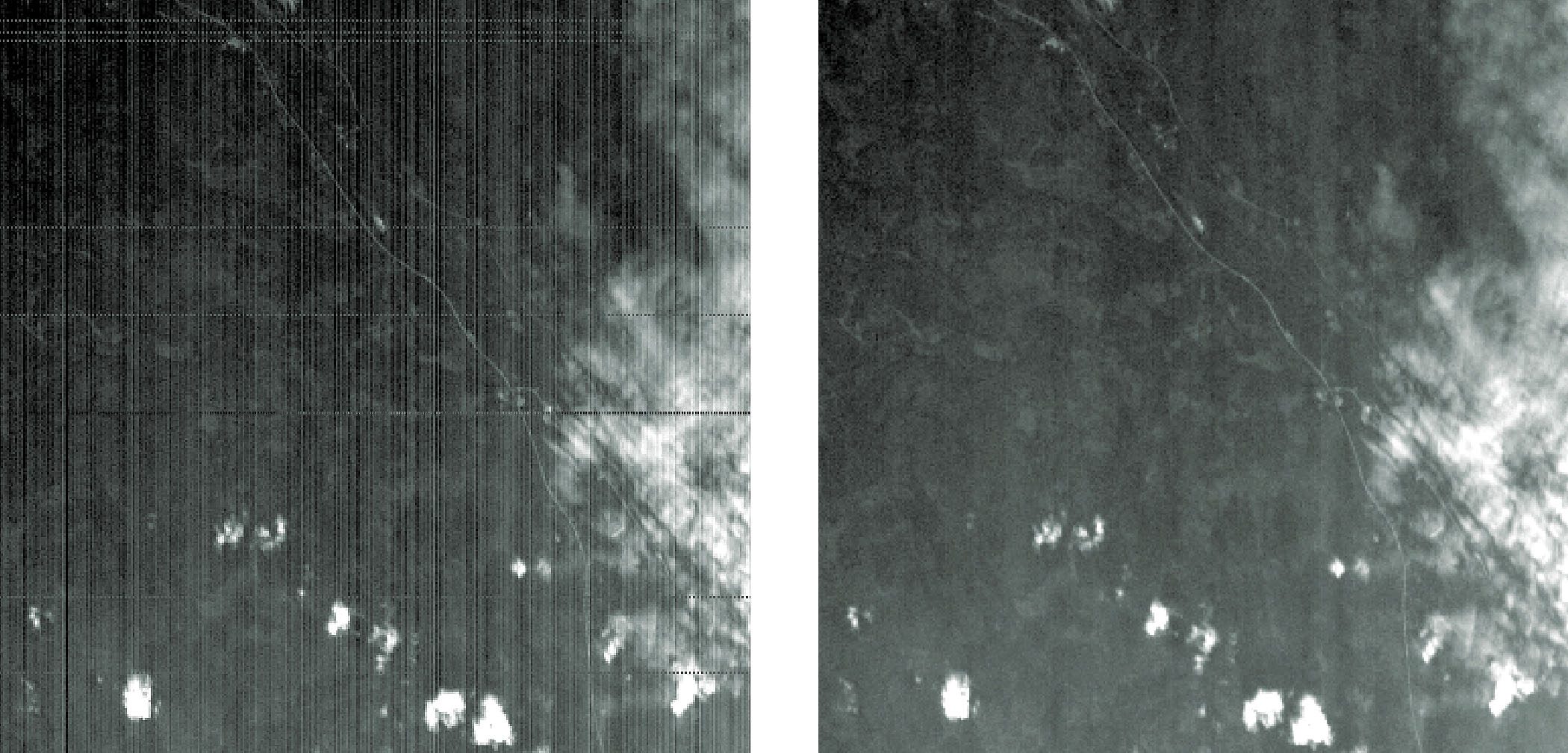
1. Noise reduction: Removes the vertical striping in CHRIS response-corrected images caused by the slit effect and a superposition of high-frequency noise
2. Cloud screening: Marks cloudy pixels in CHRIS noise-corrected images; the cloud screening algorithm provides cloud probability and abundances for each pixel
3. Atmospheric correction: Provides a surface reflectance retrieval algorithm. The method applies to noise-corrected radiance images with (or without) a probabilistic cloud mask as generated by the cloud screening algorithm
4. Geometric correction: Computes longitude and latitude coordinates (WGS-84) as well as viewing angles for each image pixel. The geometric correction is applicable to atmosphere-corrected images.
5. TOA reflectance computation: Computes top-of-atmosphere apparent reflectance from the top of atmosphere radiance (radiometrically calibrated data) as provided by the CHRIS noise-corrected images
6. Feature extraction: Computes certain surface and atmospheric features which are used by the CHRIS-Box cloud screening algorithm; the feature extraction is applicable to TOA reflectance images only

CHRIS/Proba Noise Reduction

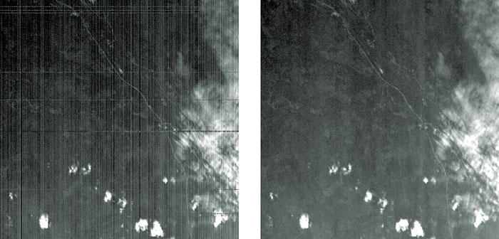
The Noise Reduction Tool is used to correct and remove the coherent noises, known as drop-outs and vertical striping, usually found in hyperspectral images acquired by push-broom sensors such as CHRIS.

Introduction

Hyperspectral images acquired by remote sensing instruments are generally affected by two kinds of noise. The first one can be defined as standard random noise, which varies with time and determines the minimum image signal-to-noise ratio (SNR). In addition, hyperspectral images can present non-periodic partially deterministic disturbance patterns, which come from the image formation process and are characterized by a high degree of spatial and spectral coherence. The objective of the Noise Reduction Tool is to correct or reduce these noise signals before any further processing.

• Drop-outs: One of the errors affecting CHRIS images is the fact that transmission of CHRIS channel 2 (odd and even pixels from each CCD row are read in parallel) randomly fails producing anomalous values at the odd pixels in some image rows called drop-outs. Drop-outs hamper the operational use of CHRIS images since latter processing stages are drastically affected by these anomalous pixels. These errors must be identified and corrected by making use of both spatial and spectral information of the anomalous pixel and its neighbors.
• Vertical striping: Another well-known problem of CHRIS images is a spatial coherent noise usually found in images acquired by push-broom sensors. This multiplicative noise in image columns comes from irregularities of the entrance slit of the spectrometer and CCD elements in the across-track direction (horizontal lines). Although the whole system was fully characterized after assembly, changes in temperature (due to the seasonal variation of the in-orbit CHRIS instrument temperature) produce a dilation of the slit that results in a complex vertical pattern dependent on the sensor's temperature, and thus it must be modeled and corrected.

Noise Reduction Algorithm

The algorithm implemented by the Noise Reduction Tool is described in detail by Gómez-Chova et al. (2008). In brief, the following steps are carried out:

Drop-out Correction

In CHRIS images, drop-outs can be seen as missing pixels with anomalous values (usually zero or negative values). These invalid values are detected and replaced by a weighted average of the values of the neighboring pixels. In order to avoid the poor performance of spatial filters (local average) in border or inhomogeneous areas, the contribution of each pixel of a given neighborhood of size 3x3, is weighted by its similarity to the corrected pixel. In particular, this similarity weight is the inverse of the Euclidean distance between the spectral signature of the pixels, which is calculated locally using the spectral bands closer to the band presenting the drop-out. It is worth noting that the values of bands with errors are not considered during this process.
The result of this process is similar to a spatial interpolation but taking into account the spectral similarity with neighbors. Although it is a cosmetic correction, it is needed since later processing stages are drastically affected by these anomalous pixel values.

Vertical Striping Correction

The objective of vertical striping correction methods is to estimate the correction factors of each spectral band to correct all the lines of this band. The main assumption consists in considering that both slit and CCD contributions change from one pixel to another (high spatial frequency) in the across-track direction but are constant in the along-track direction, i.e. during the image formation; while surface contribution presents smoother profiles (lower spatial frequencies) in the across-track dimension. Several algorithms already exist to reduce vertical striping, but most of them assume that the imaged surface does not contain structures with spatial frequencies of the same order than noise, which is not always the case. The proposed method introduces a way to exclude the contribution of the spatial high frequencies of the surface from the process of noise removal that is based on the information contained in the spectral domain.
Standard vertical striping reduction approaches take advantage of the constant noise factors in the image columns. Basically, each image's column is averaged resulting in an averaged line (along-track) and then the noise profile is estimated in the across-track direction for each band. By averaging image lines (integrated line profile) the surface contribution is smoothed, the additive random noise is cancelled, and the vertical striping profile remains constant. Consequently, the surface contribution presents lower spatial frequencies in the integrated line profile and can be easily separated from the vertical striping (high frequencies) applying a filter with a suited cut-off frequency.
One of the main drawbacks of these methods is the fact that they do not take into account the possible high frequency components of the surface explicitly. In images presenting structures or patterns in the vertical direction, the averaged profile may present high frequency contributions due to the surface. This will be interpreted as vertical striping, and some columns will be corrected with wrong values, worsening the final image. The proposed correction method is also based on the hypothesis that the vertical disturbance presents higher spatial frequencies than the surface radiance. However, it models the noise pattern by suppressing the surface contribution in the across-track in two different ways: first, avoiding the high frequency changes due to surface edges, and then subtracting the low frequency profile. In addition, thanks to the sequential acquisition of CHRIS of the same scene from five different angles, the robustness of the proposed algorithm can also be improved using together all the multiangular images of one acquisition. When processing together a higher number of lines, the surface contribution is smoother and the estimation of the vertical striping is more accurate.

Summary of the Complete Processing Chain

The optimal sequence of algorithms to be applied in order to correct a given image is the following:

• Drop-outs are detected and corrected.
• A rough correction of the vertical striping due to the entrance slit is performed. For a given CHRIS image, the estimation of the slit vertical striping is obtained from a previous characterization of the vertical striping pattern stored in a look-up-table (LUT), which includes the dependence on the platform temperature at the given CHRIS acquisition
• After the preliminary correction of the vertical striping due to the entrance slit, the robust vertical striping correction method is used to estimate directly from the image (or multiangular image set) the remaining vertical striping for each band.
• Finally, obtained vertical striping coefficients are used to correct the image column values.

L. Gómez-Chova, L. Alonso, L. Guanter, G. Camps-Valls, J. Calpe, and J. Moreno, "Correction of systematic spatial noise in push-broom hyperspectral sensors: application to CHRIS/Proba images," Appl. Opt. 47, F46-F60 (2008)

CHRIS/Proba Cloud Screening

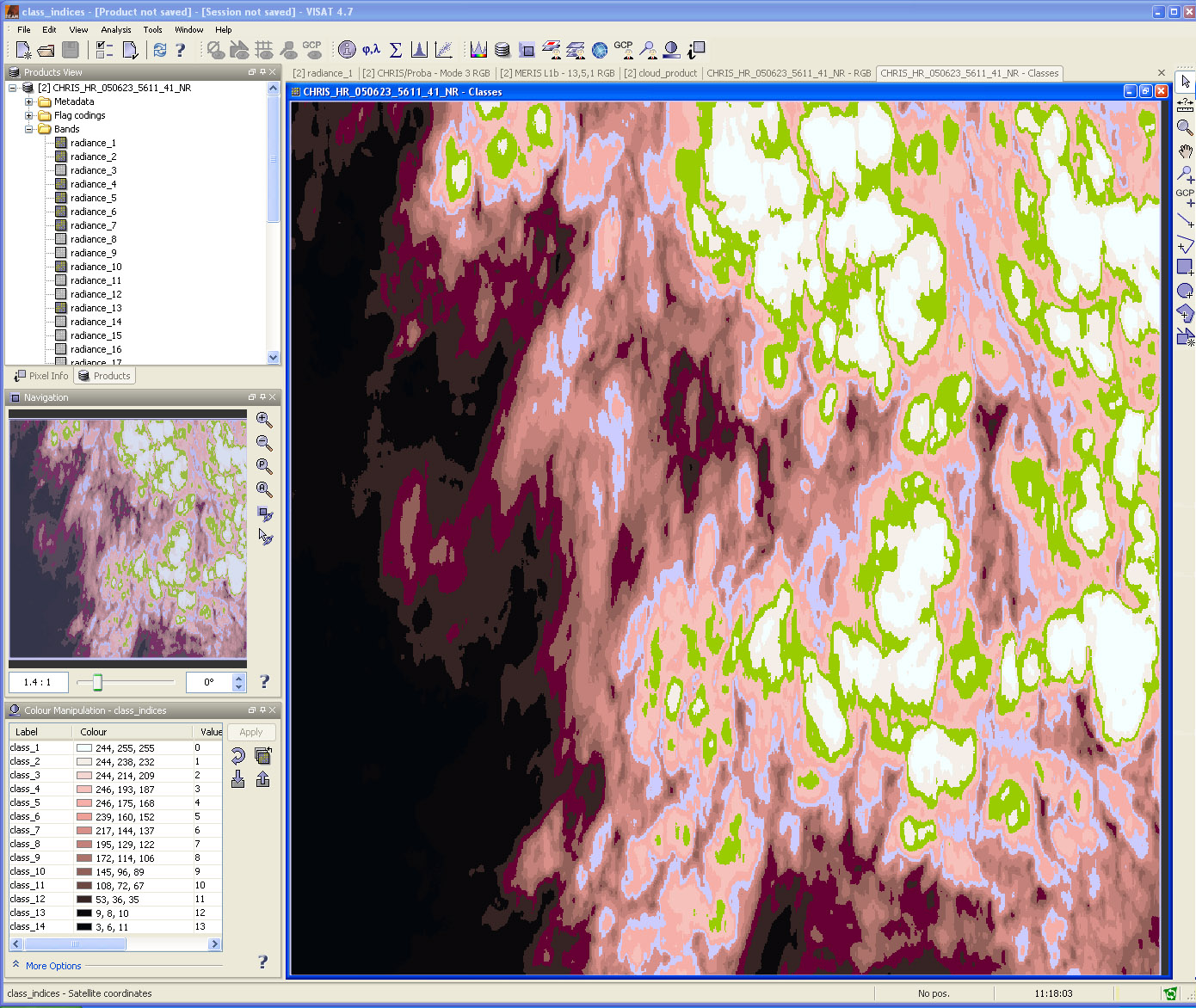
The Cloud Screening Tools is used to mask cloudy pixels in CHRIS images. The cloud masking algorithm described below helps the user to find cloudy regions in the image and provides cloud probability and abundances for each pixel instead of a single flag.

Cloud Screening Algorithm

The cloud screening algorithm consists of the following steps:

1. TOA Reflectance Computation: Top-of-Atmosphere reflectance is estimated from the CHRIS products to remove in practice the dependence on particular illumination conditions (day of the year and angular configuration).
2. Feature extraction: physically-inspired features are extracted to increase separability of clouds and surface taking into account that the measured spectral signature depends on the illumination (TOA reflectance is already estimated), the atmosphere (oxygen and water vapor atmospheric absorptions are used to estimate the optical path related to the cloud height), and the surface (spectral whiteness and brightness helps to characterize the cloud's spectral behavior).
3. Image clustering: an unsupervised Expectation-Maximization (EM) clustering algorithm is performed on the extracted features in order to separate clouds from the ground-cover while obtaining posterior probabilities of each pixel to each cluster.
4. Cluster labeling: resulting clusters are subsequently labeled by the user. Once all clusters corresponding to clouds have been identified, it is straightforward to merge all the clusters belonging to a cloud type (cloud-clusters). In the clustering of the extracted features, the EM algorithm provides a probabilistic membership for each cluster, thus the probability of being cloud is computed as the sum of the posteriors of the cloud-clusters.
5. Spectral unmixing: a Fully Constrained Linear Spectral Unmixing (FCLSU) is applied to the image in order to obtain the fraction of cloud content for each pixel (rather than flags or a binary classification).

The final cloud product is obtained combining the cloud probability and the cloud fraction by means of a pixel-by-pixel multiplication. That is, combining two complementary sources of information processed by independent methods: the cloud probability (obtained from the extracted features), which is close to one in cloud-like pixels and close to zero in remaining areas; and the cloud abundance or mixing (obtained from the spectra).

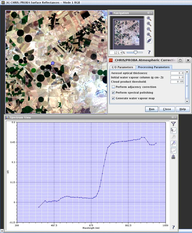
CHRIS/Proba Atmospheric Correction

Introduction

The atmospheric correction, i.e. the conversion from top-of-atmosphere (TOA) radiance to reflectance images, is one of the most important steps in the pre-processing of remote sensing data. The CHRIS Atmospheric Correction Tool converts from TOA radiance to surface reflectance images in an automated manner by means of a modular approach which involves the characterization of atmospheric and instrumental parameters.
The algorithm is implemented so that it must be applied after noise removal and cloud screening. The interface between atmospheric and geometric correction modules is not established at this stage of the project, so the correction of topographic effects with a digital elevation model are not considered in the current version of the Atmospheric Correction Tool.

Algorithm

Overview

The algorithm implemented in the Atmospheric Correction Tool is described in detail in Guanter et al. (2005a,b). In the most general processing, the following steps are carried out:

1. Update of spectral characterisation  (CHRIS modes 1 & 5)
2. Aerosol optical thickness (AOT) retrieval
3. Columnar water vapour (CWV) retrieval (CHRIS modes 1, 3 & 5)
4. Surface reflectance retrieval
5. Spectral polishing - removal of systematic errors in surface reflectance (CHRIS modes 1 & 5)

The different steps to be performed along the atmospheric correction process depend on the CHRIS acquisition mode. In particular, CWV is only derived for CHRIS acquisition modes 1, 3 and 5, as no sufficient sampling of water vapor absorption features is provided by modes 2 and 4. On the other hand, spectral calibration and an optional spectral polishing are only performed on modes 1 and 5, which are the ones providing the necessary high spectral resolution around sharp spectral features.

The different processing modules composing the CHRIS Atmospheric Correction Tool assume clear-sky conditions. Cloudy pixels are screened out from the processing using the cloud mask provided by the cloud screening module and the Cloud product threshold to be selected by the user as a processing parameter. This indicates the limit value of the probabilistic cloud mask discriminating cloudy and clear pixels. This threshold is not necessary if only a binary cloud mask was generated by the cloud screening module (no unmixing applied).

The MODerate resolution TRANsmittance (MODTRAN4) atmospheric radiative transfer code (Berk et al., 2003) was used for the generation of a Look-Up Table (LUT) which provides the atmospheric parameters  used by the different modules from multidimensional linear interpolation. MODTRAN4 has been selected for its good parameterisation of both scattering and absorption atmospheric processes, as interposed by an algorithm dealing with simultaneous aerosol and water vapor retrieval. The LUT depends on 6 free input parameters: view zenith angle, solar zenith angle, relative azimuth angle, surface elevation, aerosol optical thickness at 550 nm (AOT550) and CWV. The atmospheric vertical profile is given by the default midlatitude summer atmosphere, the aerosol type is fixed to the continental model, and the ozone concentration is fixed to 7.08 g·m−2. The LUT was generated using the New Kurucz extraterrestrial solar irradiance data base in MODTRAN4.

Update of spectral characterisation

The first step in the Atmospheric Correction Tool for modes 1 and 5 is the evaluation of potential problems in the instrument spectral calibration. The lower spectral resolution and sampling of the acquisition modes 2, 3 and 4 leads to the smaller sensitivity to spectral calibration errors in these modes.
In the case of pushbroom imaging spectrometers such as CHRIS, errors in the instrument spectral calibration are generally associated to the knowledge of the channels center wavelength, and are mostly caused by spectrometer shifts (systematic bias in channel position) and spectral smile (non-linear variation of channel position within the across-track direction of the image). The spectral response function and bandwidth are expected to have lower deviations from the laboratory calibration.
Errors in surface reflectance appear around atmospheric absorption features when the band configuration applied in the resampling of the atmospheric parameters during atmospheric correction differs from the actual one. The fundamental basis for the determination of the real wavelength position is the removal of those errors. The method for spectral characterisation in the Atmospheric Correction Tool (Guanter et al, 2006) performs an iterative search for the channel position which generates the smoothest surface reflectance spectrum after atmospheric correction. The O2 absorption feature centered at 760 nm is used as reference for the CHRIS spectral calibration. The across-track direction is represented by a set of radiance spectra derived by averaging all the spectra in the along-track direction into one single pixel for each image column. The channel spectral position is evaluated independently for each one of them in order to characterise spectral shift and smile at the 760 nm region.
However, in view of the low peak-to-peak smile detected in CHRIS (Guanter et al, 2006), and in order to speed-up the processing, atmospheric correction is not performed column-wise accounting for the exact channel position at each column, but only a mean value characterising the overall spectral shift from the nominal channel positions is used to update the later ones. The spectral shift in the 760 nm is assumed to be representative of the entire CHRIS spectral range.

AOT retrieval

Different AOT retrieval methods are applied to land and water modes. For the retrieval of AOT over land targets, the technique already described in Guanter et al. (2005) is applied. The total aerosol loading is parameterised by the AOT at 550 nm. No attempt to derive information on the aerosol model is made, but it is assumed that the aerosol optical properties are sufficiently described by the rural aerosol model implemented in MODTRAN4. It is also assumed that the AOT is constant all over the imaged area. After cloud screening, the lowest radiance value in each spectral band within the image is found. The resulting spectrum is employed as a reference dark target. It provides the highest limit for the aerosol content: an iterative procedure looks for the AOT550 value leading to the atmospheric path radiance which is closest to the radiance in the dark spectrum, not allowing path radiance to be higher than the dark spectrum in any of the visible bands (from 410 to 680 nm). The next step is refining that initial AOT550 estimation with a more sophisticated method involving the inversion of TOA radiances in combinations of green vegetation and bare soil pixels. This is performed only over those pixels which are classified as land pixels. AOT550 is then retrieved from 5 pixels with high spectral contrast inside this window, by means of a multiparameter inversion of the TOA spectral radiances in those pixels.

Please, note that only the top threshold of AOT550 is calculated by the current version of the aerosol retrieval module for CHRIS modes 1, 3, 4 and 5. The calculated top AOT value is labeled as 'Maximum AOT550' in the MPH file. An improved version of the aerosol retrieval algorithm over land including the inversion of vegetation and soil pixels will be available in future releases of the software.

In the case of inland water pixels, the particular performance of CHRIS in the mode 2 configuration (optimised for the observation of water bodies) causes that a different AOT retrieval approach must be considered. The use of land pixels is avoided for mode 2 data, due to the saturation usually found for surface albedos higher than 20-25%. The procedure described above for the land modes to set the maximum AOT value is used to calculate the final AOT value in mode 2. The AOT550 leading to the path radiance spectrum equal to or lower than the TOA radiance from the darkest pixels in the in the 435-690 nm range is selected. The first band, centered in 410 nm, is avoided because of the high noise levels detected. The final AOT550 is expected to be closer to the real value in the case of dark water bodies, from which most of the TOA signal is due to atmospheric scattering.
In the case that the user can provide a reliable AOT550 value from external sources, it can be entered in the Aerosol optical thickness at 550 nm processing parameter field. The AOT retrieval module would not be applied in this case.

CWV retrieval

Water vapor retrieval is based on a band-fitting approach making use of the water vapor absorption centred at 940 nm. Surface reflectance outside and inside the left wing of that absorption feature is assumed to be linear with wavelength for the band-fitting inversion. A real band-fitting technique is only applied to modes 1 and 5, which are the ones providing a complete sampling of the 940 nm water vapor absorption feature. In the case of the mode 3, only two bands, centered about 900 and 910 nm, are affected by that absorption. However, the inversion of these two bands following the procedure described before has shown to be sufficient for the accurate water vapor retrieval.
More accurate CWV values may be obtained if an initial value is provided to the algorithm (processing parameter Initial water vapour column (g cm^-2)). The user can also select a faster processing option (deactivating Generate water vapour map) in which water vapor retrieval is only performed on a selected subset of pixels, rather than per-pixel, the retrieved mean value been applied to the complete image. However, thanks to the efficient JAVA implementation of the code, the per-pixel CWV retrieval is recommended as default.

Surface reflectance retrieval

Reflectance images are derived from TOA radiance after AOT and CWV retrieval. AOT and pixel-wise CWV are used as inputs to the MODTRAN4 LUT for the calculation of the atmospheric parameters to be used for the radiance-to-reflectance inversion.
The resulting reflectance images can be further processed to remove the image blurring caused by those photons reflected by the target environment and scattered by the atmosphere particles into the sensor’s line-of-sight. This effect is called adjacency effect, because the apparent signal at the TOA for a given pixel comes also from the adjacent ones. The simple formulation proposed by Vermote et al. (1997) is followed here. It is based on the idea of weighting the strength of the adjacency effect by the ratio of diffuse to direct ground-to-sensor transmittance. This approach may be too simplistic in some cases (i.e. large view or illumination zenith angles, large aerosol loading) so the application of adjacency correction is performed only under user request (processing parameter Perform adjacency correction).

Spectral polishing

Systematic errors in the form of spikes and dips may appear in the surface reflectance product. Out of absorption regions these errors are mostly due to problems in the instrument gain coefficients (radiometric calibration), but inside atmospheric absorptions they can also be associated to inaccurate radiative transfer simulations. The fact that they are systematic allows the correlation with an error-free reference reflectance for the correction.
The inversion of artificial endmembers is used to provide the reference reflectance patterns. Smooth spectra are calculated by spectral unmixing of spiky spectra. Up to 50 reference spectra are extracted from the reflectance images. The selection is made from a previous classification of the area based on three Normalized Difference Vegetation Index (NDVI) categories: vegetation, bare soil and mixtures. A recalibration coefficient for each CHRIS channel is calculated by correlating the 50 pairs of spectral reflectance from the spiky and smooth spectra. The reflectance image is multiplied by these recalibration coefficients, yielding the final reflectances.
It must be remarked that the spectral polishing can lead to errors in reflectance for images where the endmembers can not reproduce the actual reflectance patterns. For this reason, the recalibration process is carried out under user request only (processing parameter Perform spectral polishing).

            

A method for the surface reflectance retrieval from PROBA/CHRIS data over land: application to ESA SPARC campaigns L. Guanter, L. Alonso, J. Moreno, IEEE Transactions on Geoscience and Remote Sensing, 43, 2908-2917, 2005a.
http://dx.doi.org/10.1109/TGRS.2005.857915

First results from the PROBA/CHRIS hyperspectral/multiangular satellite system over land and water targets L. Guanter, L. Alonso, J. Moreno, IEEE Geoscience and Remote Sensing Letters, 2, 250-254, 2005b.
http://dx.doi.org/10.1109/LGRS.2005.851542

Spectral calibration of hyperspectral imagery using atmospheric absorption features L. Guanter, R. Richter, J. Moreno, Applied Optics, 45, 2360-2370, 2006.
http://www.opticsinfobase.org/abstract.cfm?URI=ao-45-10-2360

MODTRAN4 Version 3 Revision 1 User’s Manual A. Berk, G. P. Anderson, P. K. Acharya, M. L. Hoke, J. H. Chetwynd, L. S. Bernstein, E. P. Shettle, M. W. Matthew and S. M. Adler-Golden, Technical report, Air Force Research Laboratory, Hanscom Air Force Base, MA, USA, 2003.

Atmospheric correction of visible to middle infrared EOS-MODIS data over land surface: Background, operational algorithm and validation. E. F. Vermote, N. El-Saleous, C. O. Justice, Y. J. Kaufman, J. L. Privette, L. Remer, J. C. Roger, and D. Tanré, Journal of Geophysical Research, 102:17131–17141, 1997.
http://modis.gsfc.nasa.gov/EOS/SCITEAM/ARTICLES/MST_A0199.pdf

CHRIS/Proba Geometric Correction

Introduction

CHRIS/Proba is a system designed for multi-angular image acquisition of a given target, with the capability along-track and across-track pointing increasing its overpass frequency. In order to in-crease the radiometric signal the platform performs a slow-down manoeuvre consisting in rotating while scanning to keep the target for a longer time under the sensor. Besides, the scan direction is reversed during the acquisition of the second and fourth images to reduce the acceleration needed for the operation. These characteristics introduce strong perspective distortions, especially for the first and last images with larger observation zenith angles.
Many applications require the images to be geometrically referenced and/or rectified. In particular for those that make use of multi-angular information the geometric processing must be very accurate.

Solution

The proposed approach for the geometric correction of CHRIS/PROBA is based on the parametric modelling of the acquisition process. It makes use of the satellite's position, velocity and pointing at the moment of line acquisition, projecting the line of sight onto the Earth surface to calculate the geographical coordinate of each pixel. The coordinates map can then be used for the rectification of the images, or optionally be saved to an Input Geometry (IGM) file for latter use.
Theoretically the algorithm does not require any user input as it is based on the geometry of acquisition. Unfortunately PROBA platform does have a pointing problem, which has not been identified yet. Therefore, at least one GCP per image is required in order to compensate for the de-pointing although the precision of the correction is not good enough. Three GCPs per image provide satisfactory results and nine GCPs per image result in excellent co-registration for the 5 images, for the tested cases (all in Barrax).
The choice of the orbital parametric approach is based on the especial requirements that the peculiar acquisition process of CHRIS/PROBA imposes on the other existing methods for geometric correction:

• The first one is the Ground Control Points (GCP) method, which requires a quite large number of points for an accurate geometric correction (at least 30, and more than 50 for high accuracy over flat terrain), and they need to be evenly distributed. These requirements are for each one of the images in one acquisition set.
• Another possible method is based on the photogrammetric equation applied to the five images but it makes the assumption that each image is acquired instantly from a fixed point in space, which is not CHRIS/PROBA case. In order to compensate this difference in the acquisition assumptions it is necessary the use of GCPs distributed through the image.

The overlap of the five images is not too high, around 65% (estimate) due to de-pointing, but even with perfect pointing, larger observation angles provide different spatial coverage due to perspective. Therefore the co-registration of the five images is only possible in a portion of each reducing the accuracy in the excluded areas. This makes necessary a high-resolution reference image for GCP selection.
Even if the requirements of these methods are met, there is the unsolved problem of open water targets, where it is not possible to use GCP at all, except for very few pixels in the best case. The same situation appears in the case of cloudy images, rendering useless scenes that might have still some useful portions.

• At present the geometric correction prototype has been developed to a working state. It has been tested on the Barrax test site, with Mode 1 images. But further development still is required; especially the use of a DEM for line of sight interception, which has been left for the final implementation stage in order to simplify the model while being developed. Also, a refined GCP input system needs to be included. It needs extensive testing on other sites apart of Barrax, but the corresponding telemetry needs to be provided by ESA as such data is not publicly available yet. It is also necessary to test other operation modes apart of Mode 1, especially the peculiar Mode 5.
• The inputs needed by the algorithm are: telemetry with the satellite position, velocity and image timing, target centre coordinate, local DEM (in the final version). The outputs of this algorithm consist on the coordinates map in IGM files, or the rectified images if the desired output is the rectified images, then they should be also provided. As side product, observation angles maps can be produced for each of the images.
• It must be noted that this method requires ESA to provide the corresponding telemetry for each acquisition. It is possible to use orbit propagation models in order to substitute the telemetry in case it is missing, but it has not been implemented yet.

The use of IGMs might be advantageous for reducing storage space as well as for those processing algorithms that might be computationally intensive but do not required rectified images, as the number of pixels to be processed is greatly reduced. They provide geographic location of each pixel; therefore algorithms based on coordinates can still be applied (if they accept the geographical information in this form).
Spatial correlation is a possible approach to automatically set GCPs to reduce the burden on the user but it still needs supervision on each of the points detected as it is typical to get false matches.

"Quasi-automatic Geometric Correction and Related Geometric Issues in the Exploitation of CHRIS/Proba Data", L. Alonso and J. Moreno, Proceedings of the Second CHRIS/Proba Workshop, 28-30 April 2004, ESA-ESRIN, Frascati, Italy

"Advances and Limitations in a Parametric Geometric Correction of CHRIS/Proba Data", L. Alonso, J. Moreno, Proceedings of the Third CHRIS/Proba Workshop, 21-23 March 2005, ESA-ESRIN, Frascati, Italy

Description of the Acquisition Procedure

The acquistion process has been described in detail in a Technical Note provided by ESA:

The spacecraft is oriented such the instrument line-of-sight is pointing towards the target at all time. This definition leaves one degree of freedom open; the rotation around the Line-of-sight (LOS). PROBA has adopted a convention to fully define the rotation matrix from the orbital frame (roll-pitch-yaw) to the frame defining the attitude of the spacecraft while imaging. Instead of a general sequence of three rotations, only two are used.
First, a pitch rotation is made to bring the pitch-yaw plane onto the target. Then a roll rotation (the new roll) is made to bring the LOS towards the target. This strategy effectively assumes a flat earth. The projection of the instrument slit on the ground is a straight line perpendicular to the ground track when looking straight down towards nadir. It would still be a line perpendicular to the ground track after the two above rotation if the earth were flat. However, the earth sphere effectively distorts the line.

The scanning motion is super-imposed to the above manoeuver by targeting a moving point on the earth instead of targeting always the centre of the image. This point is moving over the area to image in a plane parallel to the orbital plane, effectively rotating back and forth around the orbital axis, "buried" in the earth. In order to keep the same scanning direction for all 5 images, the rotation axis is also frozen shortly (c.f freeze time above) before the beginning of the acquisition and maintained throughout. This compromise keeps the direction of scan.

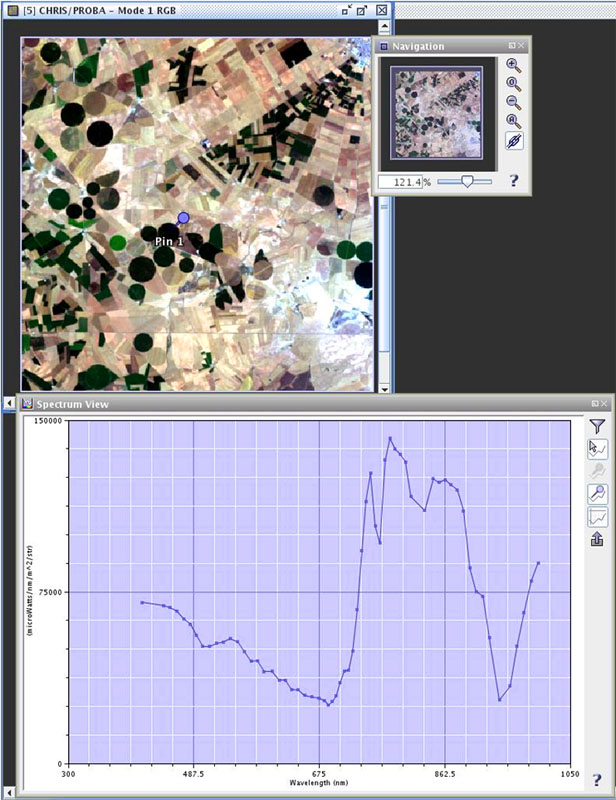
CHRIS/Proba TOA Reflectance Algorithm

CHRIS products are provided in top of the atmosphere (TOA) radiance (radiometrically calibrated data).
The TOA apparent reflectance is estimated according to:

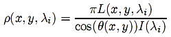
where L(x, y, λ_i) is the provided at-sensor upward radiance at the image location (x, y), I(λ_i) is the extraterrestrial instantaneous solar irradiance, and θ(x, y) is the angle between the illumination direction and the vector perpendicular to the surface.

In the proposed algorithm, θ(x, y) is approximated by the Solar Zenith Angle provided in the CHRIS attributes since one can assume flat landscape and constant illumination angle for the area observed in a CHRIS image. Finally, the Sun irradiance, I(λ,) is taken from Thuillier et al. (2003), corrected for the acquisition day, and convolved with the CHRIS spectral channels.

Thuillier, G., Hersé, M., Labs, D., Foujols, T., Peetermans, W., Gillotay, D., Simon, P. C., and Mandel, H. (2003).
The solar spectral irradiance from 200 to 2400 nm as measured by the SOLSPEC spectrometer from the ATLAS and EURECA missions. Solar Physics, 214:1�22.

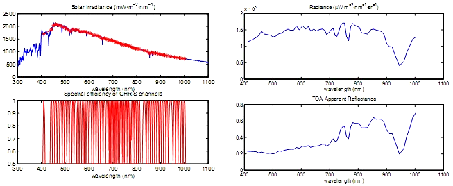
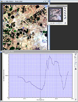
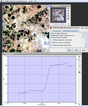
Sun irradiance corrected for the day of the year and the CHRIS channels (left) and TOA apparent reflectance estimated from the sensor radiance (right).

The extraterrestrial solar irradiance I(λ) given in Thuillier et al. (2003) is provided from 200 to 2400 nm in mW/m²/nm. It shall be corrected for the Julian day of year (DOY), J, according to the following approximate formulae:

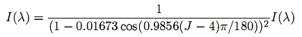
where the day of year can be easily obtained from the Image Date metadata of the CHRIS file.

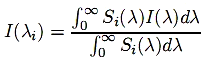
Since the reference extraterrestrial solar irradiance presents a different spectral sampling, it is resampled to the CHRIS spectral channels. A specific CHRIS band, i, consists of the addition of one or more CCD detector pixel elements depending on the band width. Therefore, the spectral response of a CHRIS band, S_i(λ,) is the sum of the the spectral response S(λ) of the corresponding detectors of the CCD array. Then, the mean solar irradiance for a given band, I(λ_i), is obtained by integrating the extraterrestrial solar irradiance by its spectral response:

The theoretical half-width of the instrument line-spread functions correspond to spectral resolutions of 1.25 nm at 415 nm, increasing to 11.25 nm at 1050 nm. One could assume a Gaussian response function, S(λ), for each element using its full-width half-maximum (FWHM), and sum up all the elements of the band. However, in the header of the CHRIS files, although the CCD row number for lower and upper wavelengths of each band is provided, the FWHM of each CCD element is not. Therefore, for the shake of simplicity, the spectral response of a CHRIS band, S_i(λ), is defined as a bell-shaped function depending on the mid-wavelength, λ_i, and the band width, Δλ_i, of the band, directly:

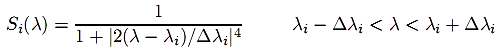
where both the mid-wavelength and the band width values for each channel are included in the CHRIS file.

CHRIS/Proba Extract Features

The Extract Features Tool is used to extract surface and atmospheric features from CHRIS images. Before you can perform the Feature Extraction on the CHRIS product, you have to apply the TOA Reflectance Computation first.

Extract Features Algorithm

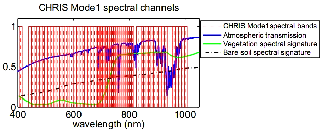
The measured spectral signature depends on the illumination, the atmosphere, and the surface. The figure below shows CHRIS Mode 1 band locations compared with the spectral curve of healthy vegetation, bare soil, and the atmospheric transmittance. The spectral bands free from atmospheric absorptions contain information about the surface reflectance, while others are mainly affected by the atmosphere.
At this step, rather than working with the spectral bands only, physically-inspired features are extracted in order to increase the separability of clouds and surface covers. These features are extracted independently from the bands that are free from strong gaseous absorptions, λi ⊂ BS, and from the bands affected by the atmosphere, λi ⊂ BA. A detailed analysis of the extracted features can be found in the ATBD.